Analyse

By using the "Analyse" function you can make simple geo-statistical analysis. As datasets you can use map layers that contain feature data. They are marked with a symbol. The function is available only for registered users.

Analyses are made with analysis methods. The available methods are described below.

Buffer

By “Buffer” method you can add a buffer around selected feature(s). You can define the buffer size yourself.

 

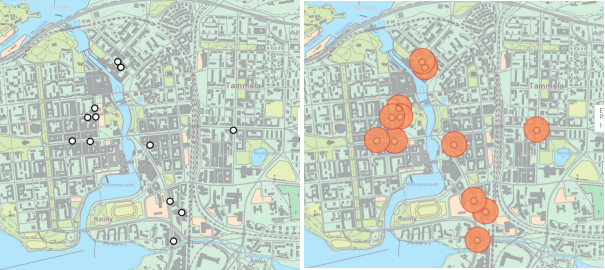
Figure. Buffers (on the right) are drawn around the features (on the right).

You can create a buffer like this:

1. Select feature(s) to which you want to make a buffer. Click a feature on the map, filter features, search places or use feature tools.
2. Select Buffer for a method.
3. Give a buffer size as meters or kilometres.
4. Select result attributes. You can select at most ten attributes. The attributes are same as in original features.
5. Type a descriptive name for the result.
6. Define a layout for result features. You can define different styles for points, lines and areas.
7. Click “Make analysis”.
8. You can see the result on the map and in the table. You can look at attribute data by clicking “Feature data” below the zoom bar.

Descriptive statistic

By “Descriptive statistic” method you can compute descriptive statistic for the selected features. Authorised features are not included in the analysis.

1. Select feature(s) for which you want to compute descriptive statistics. Click the feature on the map, filter features, search places or use feature tools.
2. Select “Descriptive statistic” for a method.
3. Select descriptive statistics to be computed:
   
   - Count: A number of the features.
   
   - Sum: The aggregate of the values.
   
   - Minimum: The smallest value.
   
   - Maximum: The biggest value.
   
   - Average: A number that describes what is the most typical value. It is computed by dividing the sum of values with the number of values.
   
   - Standard deviation: An average variation of values from the average of values.
   
   - Median: The middle number in a sorted list of numbers. If there is an even number of values, the median is an average of two middle values.
   
   - The number of authorised features: Some values are not possible to take into computation because of privacy etc. This key ratio tells the number of these values.
4. Select attributes to which descriptive statistic are computed. You can select at most ten attributes.
5. Type a descriptive name for the result.
6. Define a layout for result features. You can define different styles for points, lines and areas.
7. Click “Make analysis”.
8. You can see the result on the map and in the table. You can look at attribute data by clicking “Feature data” below the zoom bar.

Union

By “Union” method you can join the selected features in one new feature.

  

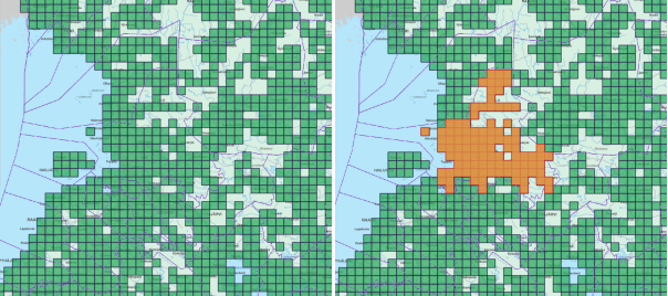
Figure. The population grid at one city has been joined in one feature. It is marked with orange at the right image. The original data is shown at the left image.

To make an union:

1. Select the features to be joined. Click a feature on the map, filter features, search places or use feature tools.
2. Select Union for a method.
3. Type a descriptive name for the result.
4. Define a layout for result features. You can define different styles for points, lines and areas.
5. Click “Make analysis”.
6. You can see the result on the map and in the table. You can look at attribute data by clicking “Feature data” below the zoom bar.

Clipping

By “Clipping” method you can clip the selected features with the features on the clipping layer. Only the features inside the features on the clipping layer are included in the result.

 

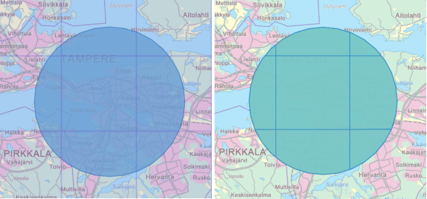
Figure. The population grid has been cut with a circular feature. The original data is at the left image.

To clip:

1. Select the features to be clipped. Click a feature on the map, filter features, search places or use feature tools.
2. Select "Clipping" as the method.
3. Select a map layer to be clipped. This map layer will be clipped with the features on the clipping layer.
4. Select a clipping map layer. The features on this map layer will cut the features on another layer.
5. Select result attributes. You can select at most ten attributes. The attributes are same as in original features.
6. Type a descriptive name for the result.
7. Define a layout for result features. You can define different styles for points, lines and areas.
8. Click “Make analysis”.
9. You can see the result on the map and in the table. You can look at attribute data by clicking “Feature data” below the zoom bar.

Geometric filter

By “Geometric filter” you can select features from the layer to be intersected. The features partially or totally inside the features on the intersecting layer are selected.

 

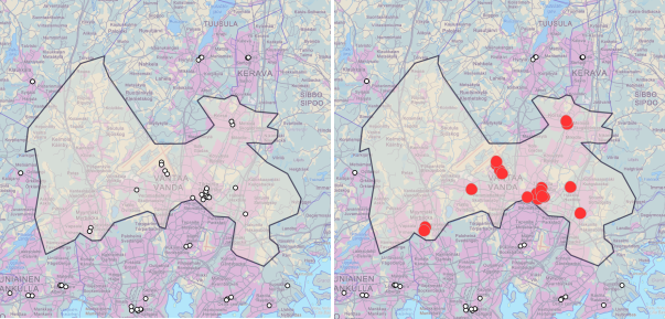
Figure. The point features (service points) are intersected with municipal divisions so that only the points in one city (Vantaa) have been filtered in the result. The result features are marked with red in the left image.

To select features inside a geometry:

1. Select the features to be filtered. Click a feature on the map, filter features, search places or use feature tools.
2. Select “Geometric filter” for a method.
3. Select an original layer. This map layer will be filtered based on the features on the intersecting layer.
4. Select an intersecting layer. The filter is based on the features on this map layer. Please note that you can filter also this map layer with a filter function in the dataset list.
5. Select result attributes. You can select at most ten attributes. The attributes are same as in original features.
6. Type a descriptive name for the result.
7. Define a layout for result features. You can define different styles for points, lines and areas.
8. Click “Make analysis”.
9. You can see the result on the map and in the table. You can look at attribute data by clicking “Feature data” below the zoom bar.

Analysis Layer Union

By “Analysis Layer Union” method you can combine the selected analysis layers. You can combine them only if they have same attributes. Original layers must be created in the analysis function. For example if you have made same analysis for two areas, you can combine those areas.

 

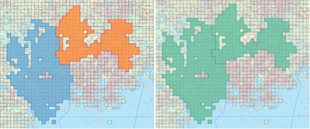
Figure. Two areas (on the left) are combined into a single area (on the right).

Näin yhdistät analyysitasoja:

1. Select an analysis layer to be combined with other analysis layer. The layer must be created in the analysis function.
2. Select “Analysis layer union” as the method.
3. Select analysis layers to be combined in the selected analysis layer. Also these layers must be created in the analysis function. All the layers must have same attributes. You can select several analysis layers.
4. Select result attributes. You can select at most ten attributes. The attributes are same as in original features.
5. Type a descriptive name for the result.
6. Define a layout for result features. You can define different styles for points, lines and areas.
7. Click “Make analysis”.
8. You can see the result on the map and in the table. You can look at attribute data by clicking “Feature data” below the zoom bar.

Buffers and Sectors

By “Buffers and sectors” method you can add several buffers and sectors around the selected features.

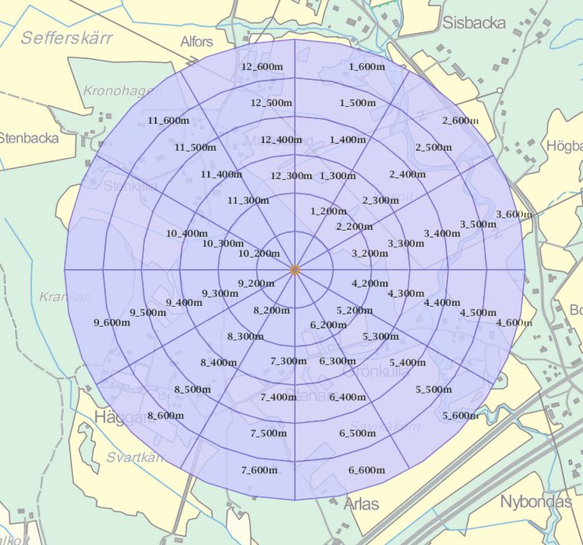
Figure. Six buffers and twelve sectors have been calculated around the point.

To calculate buffers and sectors:

1. Select feature(s) to which you want to make buffers and sectors. Click a feature on the map, filter features, search places or use feature tools.
2. Select “Buffers and sectors” for a method.
3. Give a buffer size as meters or kilometres.
4. Give a buffer amount. One feature can have at most 12 buffers.
5. Give a sector amount. One feature can have at most 12 sectors.
6. Select result attributes. You can select at most ten attributes. The attributes are same as in original features.
7. Type a descriptive name for the result.
8. Define a layout for result features. You can define different styles for points, lines and areas.
9. Click “Make analysis”.
10. You can see the result on the map and in the table. You can look at attribute data by clicking “Feature data” below the zoom bar.

Difference Computation

By “Difference computation” method you can compute a difference between two map layers. Map layers present the same location at two different times. For example you can compute how the population amount has changed during the last five years.

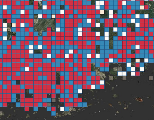
Figure. The difference in population amount between two years has been computed for the population grid in the capital area. The growth (positive change) has been marked with red and the decline (negative change) with blue.

Näin lasket muutoksen eri karttatasojen välillä:

1. Select an older map layer (t1). This layer contains original data.
2. Select “Difference computation” for a method.
3. Select a comparable attribute from the older map layer. These values are compared with data from the newer map layer.
4. Select a newer map layer (t2). This layer contains updated data.
5. Select a comparable attribute from the newer map layer. These values are compared with data from the newer map layer.
6. Select a combining attribute. It must be a unique identifier tor both of map layers.
7. Select result attributes. You can select at most ten attributes. The attributes are same as in original features.
8. Type a descriptive name for the result.
9. Define a layout for result features. You can define different styles for points, lines and areas.
10. Click “Make analysis”.
11. You can see the result on the map and in the table. You can look at attribute data by clicking “Feature data” below the zoom bar.

Spatial Join

By “Spatial join” method you can join attribute data from two different layers. Feature attributes are joined based on location.

Figure. Features at the feature level and at the source level are joined base on their location.

To create a Spatial Join:

1. Select a feature layer. Attributes from this map layer are joined with attributes from the source layer. If you want, you can filter features.
2. Select “Spatial join” for a method.
3. Select result attributes from the feature layer. These values are compared with data from the newer map layer. You can select at most ten attributes. The attributes are same as in original features.
4. Select a source layer. Attributes from this map layer are joined with attributes from the feature layer.
5. Select result attributes from the source layer. These values are compared with data from the newer map layer. You can select at most ten attributes. The attributes are same as in original features.
6. Select result features from the feature layer. You can select intersecting or containing features. Intersecting features are partially or totally inside the features at the source layer. Containing layers are totally inside the features at the source layer.
7. Select result attributes. You can select at most ten attributes. The attributes are same as in original features.
8. Type a descriptive name for the result.
9. Define a layout for result features. You can define different styles for points, lines and areas.
10. Click “Make analysis”.
11. You can see the result on the map and in the table. You can look at attribute data by clicking “Feature data” below the zoom bar.

---

Select Dataset

The list ’Datasets’ includes all the data products which are visible on the map window. You can only make analysis to the datasets including feature data (WFS). They are marked by the icon. Select one dataset to a base for your analysis. You can also search more datasets pressing “More datasets”.



You can open metadata for the dataset by clicking the button. By clicking the button you can filter datasets. You can also take off the dataset from the map window by clicking the button.

Filter Dataset

Filter features from the map layer by clicking the filter button. You can filter features geographically or based on attribute data. Only the filtered features are taken into account in the analysis.

Filter geographically: The filtered attributes are selected based on the map view area or feature selections. The result contains all features, features visible in the map view, features selected on the map, features intersecting the selected attribute or features inside the selected features.



Filter based on attribute data: The filtered attributes are selected based on the conditions you give. The condition is like “x=y”, where x is an attribute, = is an operator and y is a value. It can be for example “population < 1000”. The result contains the features satisfying the condition. You can add conditions by clicking the (+) button or take off by clicking the (-) button. You can select if the conditions are case-sensitive.



When you have selected all the filters, click “Refresh”. You can also clear all the filters by clicking “Clear All” or you can return back to analysis without saving the filters by clicking ‘Cancel’.



Focus Map

You can focus the map to the place you want. Search a place by clicking the “Search places”. You can search places based on place names, addresses or real estate identifiers. You can create a temporary point by clicking “Import to analysis”. Now you can use this point in the analysis.

Feature tools

Use feature tools to add temporary features, clip features and select features geometrically.



Add Temporary Feature to Map



Add a temporary feature. The feature can be a point, a line or an area. It can also consist of several features. The temporary feature is not saved. It will be taken off after closing Analysis function. You can use temporary features as a base for analysis.



Add a temporary point:

1. Click the location you want.
2. Repeat the 1st phase if the feature consists of several points.
3. Click “Done”. Remove point(s) by clicking “Cancel”.
4. The point is now at the dataset list. Its name is “Temporary point x”, where x is its order number.

Add a temporary line:

1. Click a starting point and breaking points. Finally double-click an ending point.
2. Repeat the 1st phase if the feature consists of several points.
3. Click “Done”. Remove line(s) by clicking “Cancel”.
4. The line is now at the dataset list. Its name is “Temporary line x”, where x is its order number.

Add a temporary area:

1. Click corner points. Finally double-click an ending point. You can make holes, if you keep ALT-key down.
2. Repeat the 1st phase if the feature consists of several points.
3. Click “Done”. Remove line(s) by clicking “Cancel”.
4. The area is now at the dataset list. Its name is “Temporary area x”, where x is its order number.

Clip features

Clip existing features. You can clip lines or areas. A line section is defined with intersection points. An area section is defined with an intersection line or an intersection area.



Clip Line with Intersection Points

1. Select a tool.
2. Click a line. Intersection points are shown on the line. They are marked with red diamonds. If the line is a circle, intersection points are on top of one another.
3. Move intersection points by dragging them with a mouse. The result is marked with red.
4. Finally click “Done”.
5. The clipped line is now at the dataset list. Its name is “Temporary line x”, where x is its order number.

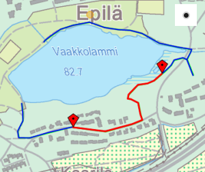
Figure. The blue line is clipped with intersection points marked with red diamonds. There is an icon for the tool in the upper right corner.

Clip Area with Intersection Line

1. Select a tool.
2. Draw a line over an area. Click breaking points (including a starting point). Finally double-click an ending point.
3. Move intersection points by dragging them with a mouse. The result is marked with blue. If you want to select the section, click another section.
4. Finally click “Done”.
5. The clipped area is now at the dataset list. Its name is “Temporary area x”, where x is its order number.
   
    

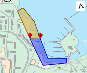
Figure. The user has drawn a line over an area. The area has been clipped based on this line. The blue area is selected. There is an icon for the tool in the upper right corner.

 

Clip Area with Intersection Area

1. Select a tool.
2. Draw an area on the selected area. Click corner points. Finally double-click a last corner.
3. Move corner points by dragging them with a mouse. The result is marked with blue. If you want to select the section, click another section.
4. Finally click “Done”.
5. The clipped area is now at the dataset list. Its name is “Temporary area x”, where x is its order number.

 

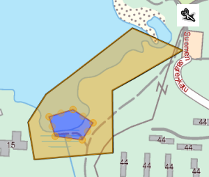
Figure. The little area has been clipped from the large area. There is an icon for the tool in the upper right corner.

Select features with Geometry

Select features by drawing a geometry around or on them. The selection is affecting only features on the selected map layer. The following geometries are available:

• Point: Click a location you want. The point is inside features to be selected.
• Line: Click breaking points (included a starting point) and double-click an ending point. Features to be selected are intersecting the line.
• Area: Click corner points. Finally double-click a last corner. Features to be selected are partially or totally inside the area.
• Rectangle: Press a mouse down and drag it from one corner to an opposite corner. Features to be selected are partially or totally inside the area.
• Circle: Press a mouse down and drag it from a focal point to a border line. Features to be selected partially or totally inside the area.

Define Layout

Define styles for features in the analysis result. The style is different for points, lines and areas:

• Points: Define a symbol, a size and a colour.
• Lines: Define a line style, a layout for heads and corners, a width and a colour.
• Areas: Define a line style, a layout for corners, a line width, a line colour and a fill colour or a fill pattern.